Power Query is all about creating a refreshable connection to a data source and making it easy for us to update the query results. However, sometimes we want to preserve those results without being replaced by future changes in the data source.
This is a common request in scenarios where we want to keep historical records or keep data unchangeable for auditing purposes. In such situations, after using Power Query to load data to a table in our Excel file, we want to prevent users from changing the information in that table by clicking “Refresh” or “Refresh All.”
Let’s see how we can disconnect a Power Query table from the data source. Stay here and learn how to break the link to source data in Power Query
Case Scenario: We have an Excel file with one query only. When we open the Queries and Connections pane from the Data tab, we see one query that connects to an external CSV file and then transforms the data and brings it into our Excel file loaded as a table.

Everyday, we run the query and save the current file as a new file named after that day’s date so that other users can have a record of what the data was on each day. However, we need to ensure that no one will hit “refresh all” and by accident changes the data that is available in the dated file. It is very much like capturing a picture of today’s data on a separate file and having it there in a static form.
Solution: There is a way to disconnect the table from the query. We will see how to do that manually and then we will use VBA to automate the repetitive work for us.
To watch my YouTube video on this topic, click here.
The manual process to disconnect the query table from the query goes like this:
Select any cell in the Excel table generated by the query and then:
- Right click and from the drop-down list, select “Table.”
- Select “Unlink from Data Source.”
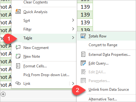
A pop-up appears with the message “This will permanently remove the query definition from the sheet. “
Click “OK.”

The Queries and Connections pane now shows “Connection only” for the query that had generated the table. Therefore, the query did not disappear and can be edited. All the steps are still available, as is the data source path.

If the user’s credentials allow him to access to the source files, and the query can be edited, the user will have access to the original data, which could be a concern in situations where there may be some confidential information stored in the source that is not visible in the final query table.
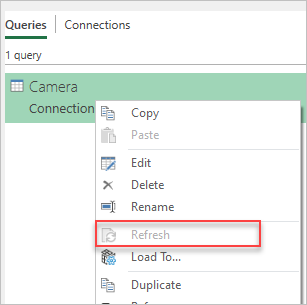
If we try to refresh the data from the table, we see that the refresh option is not available (greyed out).
However, from the query, we can do (1) “Load to” and then choose (2) “Table” and pick a destination cell (3).
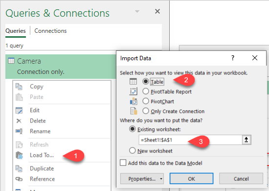
This way, we will load the data to the file again, into a new table.
Unlinking the table from the data source is not the same thing as changing the loading destination to “Connection only”. If you try to take a query that is loaded to the workbook as a Table and change its loading destination to “Connection only”, a pop up appears “This query is currently connected to a table in your workbook. Loading the query as a connection only will delete the table. Do you want to continue?”

If you say “yes”, the table disappears, and the query remains as “Connection Only.”
When you unlink the query table from the query, both the table and the connection remain in the file, but the table is no longer “refreshable” by the query.
Automating with VBA:
Although disconnecting the table from the query requires a few clicks only, having to do that manually every day plus having to save a separate copy of the file is worth taking the time to automate and transform all these steps into a one-click-only process. To do that, do as follows:
Save the file that contains the query as an Excel Macro-Enabled Workbook (* .xlsm) using the Save As and picking the type from the drop-down in the save window.
Let’s start the macro in the VBA editor by going to the developer tab and opening Visual Basic. Click “Insert” and choose “module” from the drop-down list. In that module, let’s start a new procedure by typing “Sub UnlinkTable” and then press Enter.
Let’s start by typing the list of steps we want to automate. Each step is written as a comment in the code by placing a single quote character before the text – comments are not perceived by VBA as an instruction to run.
The steps are:
‘Update the data.
‘Save the current file.
‘Save the file as workbook without macros.
‘Unlink the table in the new file
‘Save the unlinked file
You can find the complete code for this macro at the end of this blog post. The details of each code section are explained below.
The first three actions will be performed in the current workbook and then the final two actions will be performed after we save the current file as a new workbook.
The code will start:
With ThisWorkbook (meaning the one where we are writing the code)
After the first three steps, we enter “End With”
After With ThisWorkbook() entry, we update the data including all the queries and pivot tables in the workbook by adding .RefreshAll
If you just want to refresh a particular query only, then the code would have to be different.
Next, we want to save the current file using the code .Save to keep the initial file with all its content.
Then, we want to create a copy of the current file that will suffer several modifications to keep the imported data static. We need to specify that we want to save this file as a new workbook using .SaveAs and providing the full path to the file (this includes the folder, the file name and the file extension) and the file format.
ThisWorkBook.Path will generate the path to the current workbook folder.
Then concatenate with ”\”, then concatenate with a name for the new file – let’s use the time stamp using the current time and date in format, YYYY-MM-dd_hhmmss.
We don’t need the new file to have macros, so we will just save this file as an Excel file with extension .xlsx (FileFormat:=xlOpenXMLWorkbook).
To get all that, we add the code.
At this time we have the code:

After this step runs, the new file will become the active workbook. Next, the final two actions will be done with applied to the active workbook.
We place the code for those two actions in between the statements With ActiveWorkbook and End With.
How do we unlink the table?
The new workbook will be a copy of the original file containing a sheet named “Report” with the table resulting from the query. For VBA, an Excel table is a ListObject. Since we only have one table in sheet “Reports,” that ListObject index is 1.
Next, we unlink it from the source and lastly, we want to save this newly created workbook.
Let’s save our initial file containing the code that we just wrote. And then test the code by pressing F8 to run one step at a time. We are in our initial file that will be converted to a new file without macros. That’s one of the reasons why it is important to save before testing the macro.
With our file side by side with the code window, let’s run it and see how it goes.
As it runs through the steps by using F8, we should see the query updating in the Queries and Connections pane. Then, we should see the file being saved.
When pressing F8 again, we should see this file being Saved As a new file with the file format we set.
We get a message indicating that the current file cannot be saved with the macros because we are asking it to be saved as just an Excel .xlsx file format. It asks if we want to continue saving as a macro-free workbook. We say “yes”, then we are done with the current workbook that has the macros. But note that the macros are still available until we close this newly created workbook.
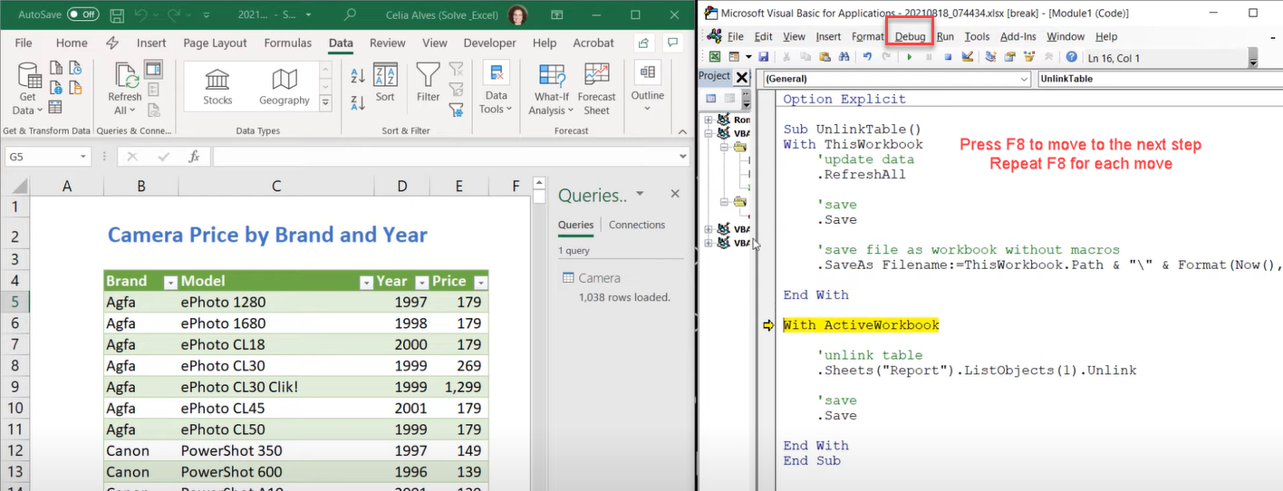
With the active workbook, we want to unlink this table from the data source. By pressing F8 again, we should see now the query in the Queries and Connections pane, change its loading destination to “connection only.”
The final step in the VBA code is to Save the file containing the unlinked table.
When we check the folder where we have the original workbook, we see that it contains the new generated .xlsx file named after the current time and date
So far, we wrote the following code:
What else can we do to improve our code?
We saw the alert message asking if we want to proceed without the macros being saved in the file, which is a bit of annoying. So we can take care of that.
Let’s reopen the original file which now has VBA and open the VBA editor.
To prevent the alert message from appearing, we add the code Application.DisplayAlerts = False just before we do the SaveAs step. But then we must re-activate the alerts after the file is saved by adding Application.DisplayAlerts = True.
Now, let’s run the code we have all at once (with F5), instead of step by step as we did before.
We will get a message “This will cancel a pending data refresh. Continue?”
So what’s going on now? The code worked fine before. Why is this happening now?
When we run all the code in one go, when it reaches the step to save the current file after refreshing the query, it happens that the step RefreshAll is not complete yet. So the file is trying to save before the query refreshing is finished.
Click Cancel. We can see that the query was not updated.
Close the file and re-open to work from the original file with the VBA code.
Let’s do those changes we need to delay the save until after the refresh completes. We need to right-click the query in the Queries and Connections pane and chose Properties. In the Query Properties dialogue window, uncheck the option “Enable background refresh”. This tells Excel that it needs to wait for the query refresh to complete before it moves on to other actions.
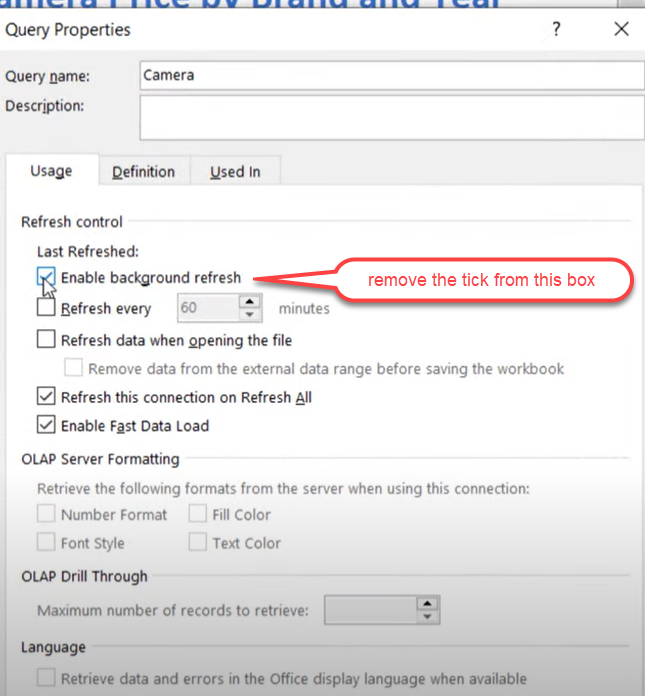
In some circumstances, this is not enough. We need to do a few other changes to our code.
Let’s add a DoEvents after the .RefreshAll step and again after each of the steps Save and Save As.
Save the VBA file and run the code.
We can see the table was unlinked from the query and the table updated correctly and it saved the file with the new file name and file format that we wanted. The alert message asking if we wanted to save the file without the macros did not appear this time and we can check that the VBA code is not available in the newly generated file.
Going back to our original file, the last step is to add a button to facilitate running this macro.
You can of course insert the shape and make a very nice button but for now we are just going to use the buttons we have under the developer tab – Insert – Button.

On the Assign Macro popup select the macro name we create (UnlinkTable).
Edit the text on the button to “Unlink Table from Source” and then save the file.
Run a final test of the code to ensure everything works.
I final detail to address would be to remove the Macro button from our final file. That file will not contain any macros, so that button is not doing anything there and might be confusing to anyone opening that file. We can accomplish this by adding one more line of VBA code: .Sheets(“Report”).Shapes.Range(Array(“Button1”)). Delete before the last .Save step.
Save the file again and test.
The complete macro code is as follows:
Saving the query results on a separate file without the query connection
It is very common that we want to save the query results separately, either to send them to other users or to use those results in other processes. And we do not want the query connection to go in that separate file containing a copy of the query results.
For that, we can copy the table range and then paste it as values and paste formattings into a new workbook.
We can program that by using with the macro recorder, while going through the steps of:
- creating a new workbook,
- selecting and copying the entire table including the headers from the workbook with the query,
- selecting a cell in Sheet1 of the new workbook and
- pasting as values and then in the same cell, pasting again selecting paste formatting.
- saving the new file an Excel.xlsx file with a file name that can be after the current date and time, and finally
- closing the new file.
- Since this Blog post is already long, I am going to just show you the code after tweaking the code generated by the macro recorder.
For full details and demo, please watch the video at the beginning of this blog post.
- Learn how to automate your Excel reports
- Get this ready-to-use Excel solution for 2 and 3 columns of Dependent Dropdown Lists
- Check other posts about Power Query and Excel in this Blog,




Leave A Comment